MMM: Workflow
Model lifecycle
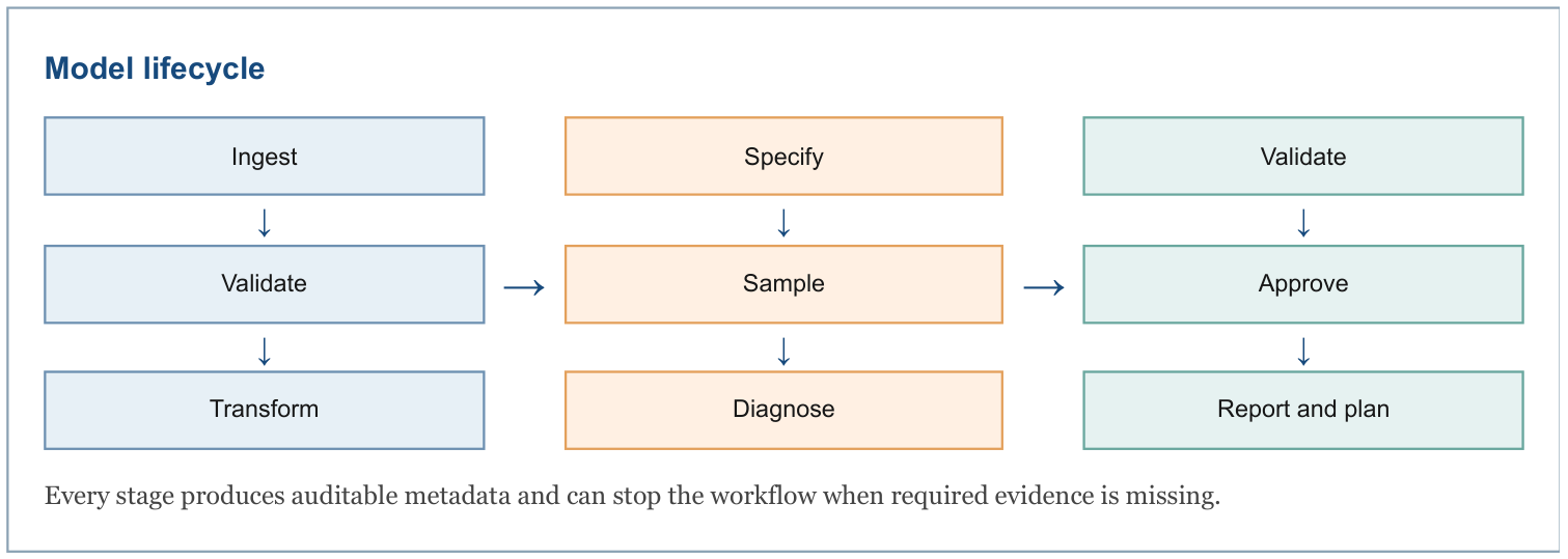
End-to-end model flow
Step 1: Ingest and classify data
Client outcome, media, spend, geography, time, control, and business-value data are mapped to a canonical schema. Ingestion validates required fields, numeric values, time grain, geography grain, media hierarchy, and semantic roles.
Step 2: Build the canonical panel
The adapter constructs aligned arrays for target , media , controls , spend , observation mask , media-to-group mapping, and business-value multipliers.
Step 3: Validate contracts and source readiness
Contracts enforce finite values, non-negative media and spend, positive business scales, contiguous group indexes, and coherent zero-spend behavior. Optional source-readiness rules validate semantic driver coverage, timestamp alignment, time grain, evidence sources, and reviewed material events.
Step 4: Diagnose identification and set adaptive pooling
The model measures activity, variation, spend support, correlations, and VIF. It converts this evidence into node-level pooling weights and attribution statuses.
Step 5: Create leakage-safe evaluation splits
The orchestration layer creates chronological train, validation, and locked-test masks, plus optional rolling-origin and balanced geography-time folds.
Step 6: Fit preprocessing on the active training mask
Exposure scales, control means and standard deviations, outcome location and scale, trend features, and baseline bases are estimated only from fitting data.
Step 7: Transform media
For every node, scaled exposure passes through the selected geometric or Weibull adstock, selected saturation family, and optional constrained neural correction.
Step 8: Construct the Bayesian model
The selected baseline, hierarchy, controls, media effects, and likelihood are assembled as an additive or multiplicative NumPyro model.
Step 9: Sample the posterior
NUTS performs warm-up and posterior sampling. JAX provides automatic differentiation, compilation, and available accelerator execution.
Step 10: Evaluate candidates
Posterior predictions are evaluated on validation and rolling folds. Sampling, predictive, peak-capture, interval, reconciliation, and identification gates are applied. Discrete candidates are ranked only after passing the configured gates.
Step 11: Refit the selected specification for locked testing
The selected model is refit on train plus validation using preprocessing learned without the test window. The locked test is used once for final evaluation.
Step 12: Test prior sensitivity and publication readiness
The active media prior is widened and attribution shares are compared. Quality flags combine sampling, predictive, source, identification, reconciliation, and sensitivity evidence.
Step 13: Produce posterior business artifacts
The reporting layer writes time-level contributions, grouped and yearly ROI, baseline/control/media decomposition, response curves where supported, prior-posterior diagnostics, holdout diagnostics, quality flags, and platform adapters. Each artifact retains uncertainty intervals and attribution metadata.
Step 14: Optional approved production refit
After an external quality decision marks the model ready and sensitivity results exist, the selected specification may be refit on all approved history. This refit does not replace the locked-test evidence; it produces the production posterior used by reporting, planning, and later-stage budget optimization.
Step 15: Later-stage budget optimization
Approved posterior response curves, contribution estimates, ROI distributions, uncertainty, and business constraints feed the budget-optimization stage. This stage evaluates allocation scenarios only after model estimation, validation, and publication-readiness checks are complete.
For the estimation and validation details behind steps 8–12, see mmm-methodology.
For the outputs produced in step 13, see mmm-results.