MMM Optimizer: Methodology

Problem statement

Let $v$ index a media vehicle (the unit the optimizer allocates to), $x_v$ its annual spend, $x_v^{0}$ its current annual spend, and $B$ the total budget. Each vehicle has a response curve $f_v(x)$ in annual units and a unit value $q_v$ (profit per unit of response).

Formula

The optimizer chooses annual spend for every vehicle to maximize total value, subject to the budget, vehicle bounds, and group shares.

$$\max_{x}\ \sum_{v} U_v(x_v) \quad \text{subject to} \quad \sum_{v} x_v = B,\qquad \ell_v \le x_v \le u_v,\qquad \underline{\omega}_g B \le \sum_{v \in g} x_v \le \overline{\omega}_g B .$$

Terms: $U_v$ is the vehicle's contribution to the chosen objective; $B$ is the total budget; $\ell_v$ and $u_v$ are the vehicle's lower and upper spend bounds; $g$ indexes a group (Traditional / Digital, or a brand); $\underline{\omega}_g$ and $\overline{\omega}_g$ are the group's minimum and maximum share of the budget.

A scenario changes only the constraints and the total budget. The same solver runs unchanged for every scenario.

---

Response curves

Every vehicle's response is a saturating function of annual spend, evaluated directly on spend. Carryover (adstock) is already embedded in the curve, so the optimizer does no time shifting.

Weibull-CDF curve (Naukr AI default)

Formula

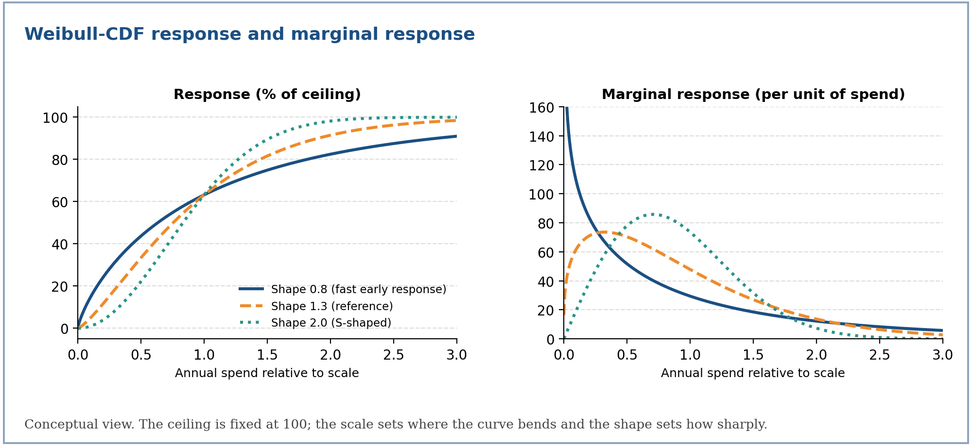
Response rises from zero toward a ceiling; the scale sets where the curve bends and the shape sets how sharply.

$$f_v(x) = \alpha_v\left[1 - \exp\!\left(-\left(\frac{x}{\kappa_v}\right)^{s_v}\right)\right],$$

Terms: $f_v(x)$ is annual incremental response at spend $x$; $\alpha_v$ is the response ceiling; $\kappa_v$ is the scale in spend units (response reaches about 63% of the ceiling at $x = \kappa_v$); $s_v > 0$ is the shape.

The spend at which the curve reaches half of its ceiling is

Formula

Half-saturation spend follows from the scale and shape.

$$h_v = \kappa_v\,(\ln 2)^{1/s_v}, \qquad f_v(h_v) = \tfrac{1}{2}\alpha_v .$$

Terms: $h_v$ is the spend giving 50% of the ceiling; $\kappa_v$ and $s_v$ are the scale and shape; $\ln 2$ is the natural logarithm of 2.

This is the same curve family as the model's own saturation. With $h$ and $k$ as in the MMM Models tab, $1 - \exp[-\ln 2\,(a/h)^{k}]$ equals the form above with $\kappa = h/(\ln 2)^{1/k}$ and $s = k$. The model fits it on normalized exposure; the optimizer needs it on annual spend, which is what the next section builds.

Hill curve (compatible engines)

Curves fitted by other supported engines use the Hill family, and the optimizer accepts both:

Formula

Hill saturation on spend.

$$f_v(x) = \alpha_v\,\frac{x^{s_v}}{x^{s_v} + k_v^{\,s_v}},$$

Terms: $\alpha_v$ is the ceiling; $k_v$ is the half-saturation spend, $f_v(k_v) = \tfrac{1}{2}\alpha_v$; $s_v > 0$ is the shape. A shape above 1 gives an S-curve; a shape of 1 or below is concave from the origin.

Marginal response: the optimization signal

The optimizer climbs the marginal response, the exact analytic derivative of the curve. There is no finite differencing and no sampling.

Formula

Marginal response of the next unit of spend, for each family.

$$f_v'(x) = \alpha_v\,\frac{s_v}{\kappa_v}\left(\frac{x}{\kappa_v}\right)^{s_v-1}\exp\!\left(-\left(\frac{x}{\kappa_v}\right)^{s_v}\right) \quad\text{(Weibull-CDF)}, \qquad f_v'(x) = \alpha_v\,\frac{s_v\,k_v^{\,s_v}\,x^{s_v-1}}{\left(x^{s_v}+k_v^{\,s_v}\right)^{2}} \quad\text{(Hill)}.$$

Terms: $f_v'(x)$ is the change in annual response per extra unit of spend; the other symbols are the curve parameters above. A tiny spend floor keeps the derivative finite at zero spend for shapes below 1.

Average ROI is reported to humans but is never the objective:

Formula

Derived business metrics for a vehicle at spend $x$.

$$\mathrm{ROI}^{avg}_v(x) = \frac{q_v\, f_v(x)}{x}, \qquad \mathrm{ROI}^{mar}_v(x) = q_v\, f_v'(x), \qquad \sigma_v(x) = \frac{f_v(x)}{\alpha_v}.$$

Terms: $\mathrm{ROI}^{avg}_v$ is average return per dollar; $\mathrm{ROI}^{mar}_v$ is the return of the next dollar; $q_v$ is profit per unit of response; $\sigma_v$ is the saturation ratio, the share of the ceiling already reached.

---

From the Bayesian model to optimizer curves

The MMM fits response on normalized exposure (a multiple of each media node's typical execution level). The optimizer needs annual spend per vehicle. A bridge rebuilds each vehicle's spend-space curve from the approved model and registers it as a Weibull-CDF curve.

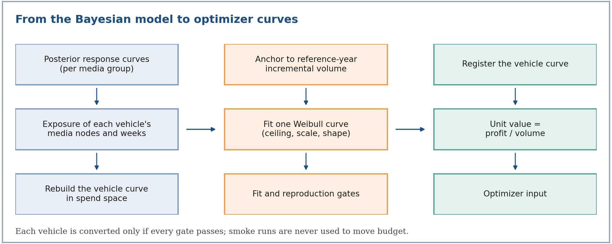
1. Group curves. For each pooling group $p$, take the published posterior-median half-response point $h_p$ and shape $k_p$, and the group's response share

Formula

The model's own response share at normalized exposure $z$.

$$S_p(z) = 1 - \exp\!\left[-\ln 2\left(\frac{z}{h_p}\right)^{k_p}\right].$$

Terms: $S_p(z)$ is the response share between zero and one; $z$ is exposure as a multiple of the node's typical level; $h_p$ is the 50% response point; $k_p$ is the shape.

The published parameters are used directly when they reproduce the published mean curve to within 2% of the ceiling; otherwise they are refitted from the published curve points.

2. Vehicle curve. A vehicle is a set of media nodes and weeks. Scaling the vehicle's spend by a multiplier $m$ scales every node's exposure by $m$, so

Formula

Vehicle response at spend multiplier $m$, anchored to the reference-year incremental volume.

$$R_v(m) = V_v\,\frac{\sum_{i \in I_v} S_{p(i)}\!\left(m\,u_i\right)}{\sum_{i \in I_v} S_{p(i)}\!\left(u_i\right)}, \qquad u_i = \frac{\text{exposure}_i}{\text{typical exposure of node}(i)} ,$$

Terms: $R_v(m)$ is the vehicle's annual response when spend is $m$ times the reference level; $V_v$ is its reported incremental volume in the reference year; $I_v$ is the set of node-week cells with positive exposure in that year; $p(i)$ is the pooling group of cell $i$; $u_i$ is the cell's exposure relative to its node's typical level (the median positive exposure over the history).

The curve is evaluated on a grid of 61 multipliers from 0 to 3, at spend $x = m\,s_v$ where $s_v$ is the vehicle's reference-year spend.

3. Single Weibull in spend space. One Weibull-CDF is fitted to those points, with the ceiling at least the largest response on the grid, the scale between 2% and 50 times the reference spend, and the shape between 0.5 and 6.

4. Unit value. The profit basis comes from the same reference year:

Formula

Profit per unit of response.

$$q_v = \frac{\text{Profit}_v}{V_v}.$$

Terms: $q_v$ is the unit value used by the profit objective; $\text{Profit}_v$ and $V_v$ are the vehicle's incremental profit and incremental volume in the reference year.

Reference year. The latest complete year: the latest year whose total spend is at least 80% of the median year's total spend.

Quality gates. A vehicle is registered only if all of these hold:

Gate	Threshold
Each group's published curve follows the model's own form	Maximum gap at most 2% of the ceiling
The vehicle curve is well described by one Weibull	Maximum gap at most 3% of the vehicle's yearly response
The registered curve reproduces the reported outcome at current spend	Difference at most 3%
Shape stays in a stable range	Between 0.5 and 6
The vehicle had positive incremental volume and profit and execution in the reference year	Required

A run is optimizable only when every vehicle that spent in the reference year converts cleanly, and only when it is a production run. A smoke (non-production) run publishes curves for display but is never used to move budget.

Assumptions recorded with every conversion: spend and exposure move together; saturation is evaluated on the period's exposure, with carryover not re-simulated; a node's typical level is the median of its positive exposure over the whole history.

---

Objective functions

The objective is a sum over every vehicle of every brand in the solve.

Formula

Per-vehicle contribution for each objective.

$$U_v^{volume}(x) = f_v(x), \qquad U_v^{revenue}(x) = p_v\, f_v(x), \qquad U_v^{profit}(x) = q_v\, f_v(x) - x .$$

Terms: $p_v$ is revenue per unit of response (it defaults to $q_v$ when no price is set); $q_v$ is profit per unit of response; $x$ is the vehicle's spend.

The gradient of each contribution is the marginal response scaled the same way ($f_v'$, $p_v f_v'$, or $q_v f_v' - 1$), so the objective and its gradient always share one basis.

Because the budget constraint fixes $\sum_v x_v = B$, the profit objective equals $\sum_v q_v f_v(x_v) - B$. For a given budget, the profit and margin-weighted revenue objectives therefore choose the same allocation; the profit objective value is simply reported net of spend.

---

What an optimum looks like

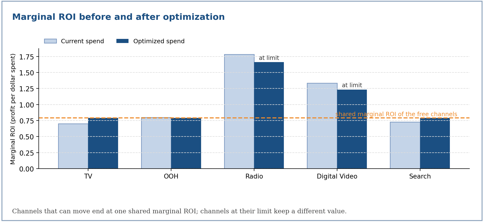
Attach a multiplier $\lambda$ to the budget constraint. At an optimum, the first-order conditions say that every vehicle that is free to move earns the same marginal value, and every vehicle held at a bound is on the correct side of it.

Formula

First-order (equal-marginal-return) conditions at the optimum, for the profit objective.

$$q_v\, f_v'(x_v^{*}) = \lambda \quad \text{if } \ell_v < x_v^{*} < u_v, \qquad q_v\, f_v'(x_v^{*}) \le \lambda \quad \text{if } x_v^{*} = \ell_v, \qquad q_v\, f_v'(x_v^{*}) \ge \lambda \quad \text{if } x_v^{*} = u_v .$$

Terms: $x_v^{*}$ is the optimal spend; $\lambda$ is the common marginal return implied by the budget; $\ell_v$ and $u_v$ are the bounds. With a binding group-share constraint, the vehicles in that group share a value shifted by that constraint's multiplier. This is a standard consequence of the Lagrangian, not an extra rule in the solver.

This is why the result is explainable: a vehicle sitting at its upper bound with a marginal ROI above the shared value is being held back by a guardrail, and loosening that guardrail would raise the objective.

For S-shaped curves ($s > 1$) the problem is not concave, so these conditions identify a local optimum. The solver safeguards below, and the validation gates, exist to catch the failure modes this creates.

---

Constraints and bounds

Vehicle bounds

For each vehicle, in this order of precedence:

1. Locked vehicles are pinned at current spend: $\ell_v = u_v = x_v^{0}$.
2. Otherwise start from the hard guardrails $m_v^{\min}$ (default 0) and $m_v^{\max}$ (default unbounded).
3. Narrow by the scenario's change limits.
4. If the result is inverted, collapse to the upper bound.

Formula

Effective bounds for an unlocked vehicle.

$$\ell_v = \max\!\left(m_v^{\min},\ x_v^{0}\,(1-\delta^{-})\right), \qquad u_v = \min\!\left(m_v^{\max},\ x_v^{0}\,(1+\delta^{+})\right).$$

Terms: $x_v^{0}$ is current spend; $\delta^{-}$ and $\delta^{+}$ are the allowed decrease and increase as fractions of current spend; $m_v^{\min}$ and $m_v^{\max}$ are hard dollar limits.

Budget and feasibility

The budget is an equality constraint, $\sum_v x_v = B$. Before solving, the optimizer checks that the problem is feasible:

Formula

Pre-solve feasibility check.

$$\sum_v \ell_v \;\le\; B \;\le\; \sum_v u_v .$$

Terms: $\sum_v \ell_v$ is the smallest total the bounds allow; $\sum_v u_v$ is the largest. If the budget falls outside, the run stops with a plain-language error that says to reduce a pinned vehicle's change, unlock a vehicle, or change the budget.

Group shares

A group $g$ (Traditional, Digital, or a brand) is constrained as a share of the budget: $\underline{\omega}_g B \le \sum_{v\in g} x_v \le \overline{\omega}_g B$. Both limits are enforced natively by the solver.

---

From a business request to constraints

The same mapping is used for every surface (see the Single Brand and Cross Brand tabs for the group and brand layers).

Total budget

The requested change applies to the movable slice of the budget; locked spend is added back unchanged.

Formula

Target total budget for a requested change $p$.

$$B = L + R\,(1 + p),$$

Terms: $L$ is the current spend of locked vehicles; $R$ is the current spend of unlocked (reallocatable) vehicles; $p$ is the requested change as a fraction (positive for an increase, negative for a decrease, zero for no change).

Applying $p$ to the full current total instead would demand that the movable slice absorb a disproportionately large change whenever much of the budget is locked.

Default vehicle guardrail

Vehicles without an explicit limit get a hard default of $\pm g$ with $g = 15\%$. The guardrail widens only if the budget itself moves further than $g$, otherwise the target would be unreachable.

Formula

Default guardrail, widened only when the budget moves more than the default.

$$\rho = \frac{B - L}{R}, \qquad \delta^{+} = \max\!\left(g,\ \rho - 1\right), \qquad \delta^{-} = \max\!\left(g,\ 1 - \rho\right).$$

Terms: $\rho$ is the ratio of the target movable budget to the current movable budget; $g$ is the default guardrail (15%); $\delta^{+}$ and $\delta^{-}$ are the effective increase and decrease limits.

Explicit vehicle limits

Request	Meaning
Increase 0, decrease 0	No explicit limit; the default guardrail applies
Only an increase or only a decrease	A directional target: the vehicle is pinned to exactly $x_v^{0}(1 \pm p)$
Both an increase and a decrease	A range: $\left[x_v^{0}(1-d),\ x_v^{0}(1+i)\right]$

---

The solver

The problem is solved with sequential least squares programming (SLSQP) using the exact analytic gradient.

Normalization. Raw spend is around ten million, which flattens the objective in the saturated regime and makes SLSQP stall. The solve runs in budget-normalized space $y = x / S$ with $S = \max(B, 1)$, so variables are of order 0.1 and the budget equality is of order 1. The objective, gradient and constraints are converted in kind (the chain-rule factor cancels exactly in the gradient).

Feasible start. The starting point clamps current spend into the bounds, then redistributes the remaining budget into vehicles with headroom (or out of vehicles with room), for up to 64 passes.

Settings. At most 300 iterations, with a function tolerance of $10^{-9}$.

Stall recovery. SLSQP can report success after a single iteration while having moved essentially nowhere. A stall is detected when the solve took at most one iteration, moved less than $10^{-6}$ from its start, and some vehicle actually had freedom to move. The solver then retries from the start nudged along its own gradient:

Formula

Restart point after a detected stall.

$$x^{retry} = x^{0} + 0.10\,\frac{B}{N}\,\hat{d}, \qquad \hat{d} = \frac{\nabla U(x^{0})}{\max_v \left|\nabla U_v(x^{0})\right|},$$

Terms: $x^{0}$ is the original feasible start; $N$ is the number of vehicles; $\hat{d}$ is the ascent direction scaled to unit maximum. The retry is adopted only if it moved, converged, met the budget equality, and reached an objective at least as good as the stalled solution, so recovery can never make a result worse.

Each iteration's objective and spend are recorded, so a run shows the objective climbing toward the optimum.

---

Diagnostics and validation

Saturation zones

Each vehicle is labelled by how much of its ceiling it has reached. The band edges are an internal rule, not universal constants.

Saturation ratio $\sigma_v$	Zone
Below 0.10	Threshold
Below 0.45	Growth
Below 0.70	Optimal
Below 0.90	Diminishing
0.90 and above	Saturation

Per-vehicle rows

For every vehicle the output reports current and optimized spend, the change in dollars and percent, current and optimized response, average and marginal ROI, the saturation ratio, the zone, and whether the optimum sits on its lower or upper bound.

Validation gates

Five checks run on every solution and are published in the summary:

Gate	Passes when
Budget equality	Total optimized spend equals the budget within a relative tolerance of $10^{-4}$
Bounds respected	Every vehicle lies inside its own bounds
Locked unchanged	Every locked vehicle still equals its current spend
Marginal declines	Marginal response does not rise as spend grows, checked only past 50% saturation (below that, an S-curve legitimately rises)
Solver success	The solver reported convergence

---

Weekly flighting

The solver produces one annual number per vehicle. The flighting engine phases it into 52 weeks.

Historical-share phasing

Formula

Each vehicle's annual optimum is phased by its own historical weekly share.

$$w_{v,t} = \frac{h_{v,t}}{\sum_{t'} h_{v,t'}}\; x_v^{*},$$

Terms: $w_{v,t}$ is the planned spend for vehicle $v$ in week $t$; $h_{v,t}$ is that vehicle's historical spend in week $t$; $x_v^{*}$ is its optimized annual spend. A vehicle with no history is phased flat at $x_v^{*}/52$. Without a historical file, every vehicle is phased flat.

Efficiency tilt

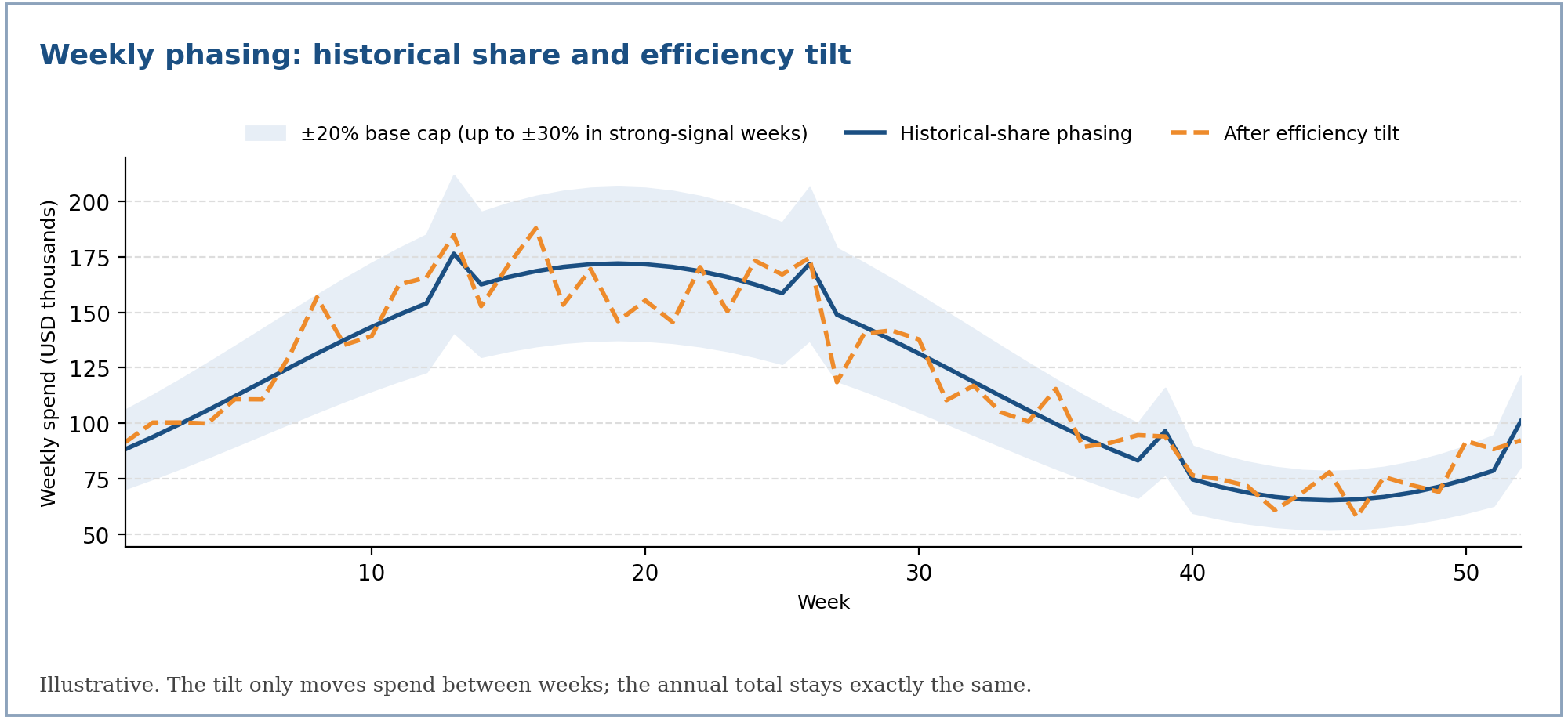
When the model provides per-week attribution, spend is tilted toward weeks that were historically more efficient, then rescaled so the annual total is unchanged.

Formula

Weekly efficiency, tilt, and per-week cap.

$$e_{v,t} = \frac{\mathrm{MaCo}_{v,t}}{\mathrm{Spend}_{v,t}}, \qquad \rho_{v,t} = \frac{e_{v,t}}{\bar{e}_v}, \qquad \tilde{w}_{v,t} = w_{v,t}\,\rho_{v,t}^{\,0.3},$$$$\gamma_{v,t} = 1 + 0.5\left(1 - e^{-0.5\,\left|\ln \rho_{v,t}\right|}\right), \qquad \left|\hat{w}_{v,t} - w_{v,t}\right| \le 0.20\,\gamma_{v,t}\, w_{v,t}, \qquad \sum_t \hat{w}_{v,t} = x_v^{*} .$$

Terms: $\mathrm{MaCo}_{v,t}$ is the model's own attributed contribution in week $t$; $\bar{e}_v$ is the vehicle's average efficiency (ratio of sums); $\rho_{v,t}$ is the week's efficiency relative to average; the exponent 0.3 keeps the tilt gentle (a ratio of 2 scales a week by about 1.23); $\gamma_{v,t}$ widens a week's cap from 1 to at most 1.5 times the base cap when its signal is strong; $\hat{w}_{v,t}$ is the final weekly spend.

A vehicle needs at least 8 weeks with positive attribution and spend before it is tilted at all; otherwise it keeps its historical-share phasing unchanged.

Aggregate weekly cap

A second, cross-vehicle cap bounds each week's combined spend against that week's historical combined spend:

Formula

Aggregate weekly band.

$$(1-0.15)\, H_t \;\le\; \sum_v \hat{w}_{v,t} \;\le\; (1+0.15)\, H_t, \qquad H_t = \sum_v h_{v,t}.$$

Terms: $H_t$ is the historical combined spend in week $t$; $\hat{w}_{v,t}$ is each vehicle's planned spend. Violating weeks are scaled to the nearest edge, and each vehicle's other weeks are rescaled to restore its annual total, for up to 5 rounds.

A feasibility guard runs first. If the optimized annual total already falls outside the sum of every week's band (for example a large annual increase phased into 52 weeks each capped at 15%), no weekly plan can satisfy both, so the cap is skipped rather than silently dropping budget. The annual decision made by the solver always wins.

---

Reporting metrics

The detailed media analysis is built from the optimized spend and the curves.

Formula

Reported metrics for a vehicle or any aggregate.

$$\text{Gross revenue} = p \times V, \qquad \text{Profit} = q \times V, \qquad \mathrm{ROI} = \frac{\text{Profit}}{\text{Spend}}, \qquad \text{Cost per unit} = \frac{\text{Spend}}{V},$$

Terms: $p$ is price (revenue per unit); $q$ is margin (profit per unit); $V$ is response volume at the shown spend. ROI here is profit over spend, not revenue over spend.

Macro assumptions. Media-cost inflation (CPM) and price inflation apply to the optimized, forward-looking side only; the current column is always the untouched historical reference:

Formula

Macro adjustment of the optimized side.

$$V^{opt} \leftarrow \frac{V^{opt}}{1 + c}, \qquad p^{opt} \leftarrow p\,(1 + \pi), \qquad q^{opt} \leftarrow q\,(1 + \pi),$$

Terms: $c$ is the net media-cost inflation (increase minus decrease): more cost means fewer response units per dollar; $\pi$ is the net price inflation, which raises value per unit.

---

Assumptions and limits

Assumption	Consequence
Carryover is embedded in each curve	The optimizer does not re-simulate adstock; weekly plans phase by history, not by model
Annual spend maps to annual response	Curves are fitted and compared on an annual basis
One fitted mean curve per vehicle	Credible bands are published for display; they do not enter the solve
S-shaped curves are not concave	The result is a local optimum; the gates report convergence and validity
Guardrails are business inputs	A vehicle at a bound is a decision to review, not a modeling result