MMM: Models

Notation and core mathematical specification

Let:

• $t \in \{1,\dots,T\}$ index time;
• $g \in \{1,\dots,G\}$ index geography;
• $r \in \{1,\dots,R\}$ index a resolved media node;
• $p(r) \in \{1,\dots,P\}$ map media node $r$ to a parent pooling group;
• $c \in \{1,\dots,C\}$ index a control variable;
• $y_{tg}$ be the modeled outcome;
• $x_{tgr}$ be raw media execution or exposure;
• $s_{tgr}$ be media spend;
• $u_{tgc}$ be a control value;
• $q_{tg}$ be profit or business value per modeled KPI unit;
• $M_{tg}$ be the observation mask.

Leakage-safe preprocessing

For media node $r$, the exposure scale is the median positive exposure in the fitting data:

Formula

Typical media exposure equals the middle positive exposure in the fitting data. Scaled exposure equals raw exposure divided by that typical exposure.

$$d_r = \mathrm{median}\{x_{tgr} : x_{tgr} > 0,\ M_{tg} = 1\}, \qquad \tilde{x}_{tgr} = \frac{x_{tgr}}{d_r}.$$

Terms: $d_r$ is the typical positive exposure for media node $r$; $x_{tgr}$ is raw exposure at time $t$, geography $g$, and media node $r$; $M_{tg}$ marks observations included in fitting; $\tilde{x}_{tgr}$ is scaled exposure.

Controls use fitting-period means and standard deviations:

Formula

Standardized control equals the control value minus its fitting-period average, divided by its fitting-period standard deviation.

$$z_{tgc} = \frac{u_{tgc} - \bar{u}_c}{s_c}.$$

Terms: $z_{tgc}$ is the standardized control; $u_{tgc}$ is the raw control value; $\bar{u}_c$ is its fitting-period mean; $s_c$ is its fitting-period standard deviation; $c$ identifies the control.

The additive outcome is standardized with fitting-period location $\bar{y}$ and scale $s_y$:

Formula

Standardized outcome equals the observed outcome minus its fitting-period average, divided by its fitting-period standard deviation.

$$\tilde{y}_{tg} = \frac{y_{tg} - \bar{y}}{s_y}.$$

Terms: $\tilde{y}_{tg}$ is the standardized outcome; $y_{tg}$ is the observed outcome; $\bar{y}$ is the fitting-period mean outcome; $s_y$ is its fitting-period standard deviation.

All preprocessing statistics are learned only from the active fitting mask. A final evaluation refit uses train plus validation and continues to exclude the locked test. An approved production refit can use all available history.

Baseline predictor

The shared scaled baseline is

Formula

Baseline demand equals the overall level plus geography and time effects plus the combined effects of all controls.

$$b_{tg} = \alpha + a_g + \tau_t + \sum_{c=1}^{C} \gamma_c z_{tgc},$$

Terms: $b_{tg}$ is scaled baseline demand; $\alpha$ is the global intercept; $a_g$ is the geography offset; $\tau_t$ is the time-related baseline effect; $\gamma_c$ is control $c$'s coefficient; $z_{tgc}$ is its standardized value; $C$ is the number of controls.

where $\alpha$ is the global intercept, $a_g$ is a partially pooled geography offset, $\tau_t$ is the selected trend, seasonality, or dynamic baseline contribution, and $\gamma_c$ is a control coefficient.

Transformed media response

For each media node, the model constructs

Formula

Transformed media response equals scaled exposure after carryover, diminishing returns, and any approved constrained correction.

$$r_{tgr} = N_{p(r)}\!\left(S_{p(r)}\!\left(A_r(\tilde{x}_{\cdot gr})_t\right)\right),$$

Terms: $r_{tgr}$ is the transformed media response; $A_r$ is the adstock or carryover function; $S_{p(r)}$ is the saturation function; $N_{p(r)}$ is the identity or constrained neural correction; $p(r)$ maps node $r$ to its parent group; $\tilde{x}_{\cdot gr}$ is the scaled exposure history.

where $A_r$ is adstock, $S_{p(r)}$ is saturation, and $N_{p(r)}$ is either the identity mapping or the constrained neural correction. Parameters may be fixed or estimated and can be scoped to each media node or its parent group as allowed by the specification.

Additive outcome model

The expected outcome in original modeled-KPI units is

Formula

Expected outcome equals restored baseline demand plus the contribution from every media node.

$$\mu_{tg} = \bar{y} + s_y\, b_{tg} + \sum_{r=1}^{R} \beta_r\, r_{tgr}.$$

Terms: $\mu_{tg}$ is the expected outcome; $\bar{y} + s_y b_{tg}$ restores the baseline to outcome units; $\beta_r$ is media node $r$'s effect coefficient; $r_{tgr}$ is the transformed response; $R$ is the number of media nodes.

Equivalently, on the standardized likelihood scale:

Formula

Standardized expected outcome equals scaled baseline plus media contributions expressed in standardized outcome units.

$$\tilde{\mu}_{tg} = b_{tg} + \frac{1}{s_y} \sum_{r} \beta_r\, r_{tgr}.$$

Terms: $\tilde{\mu}_{tg}$ is the standardized expected outcome; $b_{tg}$ is the scaled baseline; $s_y$ is the outcome standard deviation; $\beta_r r_{tgr}$ is media node $r$'s contribution in outcome units.

Media contributions add exactly to total media lift:

Formula

A node's contribution equals its effect times its transformed response. Total media lift is the sum of all node contributions.

$$C_{tgr} = \beta_r\, r_{tgr}, \qquad C^{media}_{tg} = \sum_{r} C_{tgr}.$$

Terms: $C_{tgr}$ is the contribution from media node $r$; $\beta_r$ is its effect coefficient; $r_{tgr}$ is its transformed response; $C^{media}_{tg}$ is the total media contribution.

Multiplicative log-link outcome model

The multiplicative form requires positive fitting outcomes. It builds a business baseline on the log scale:

Formula

Log baseline equals the restored scaled baseline. A media node's log lift equals its effect times its transformed response.

$$\eta^{base}_{tg} = \bar{\ell} + s_\ell\, b_{tg}, \qquad \ell_{tgr} = \beta_r\, r_{tgr},$$

Terms: $\eta^{base}_{tg}$ is the log baseline; $\bar{\ell}$ and $s_\ell$ are the fitting-period mean and standard deviation of the log outcome; $b_{tg}$ is the scaled baseline; $\ell_{tgr}$ is node $r$'s log lift; $\beta_r$ and $r_{tgr}$ are its effect and transformed response.

Formula

Total expected log outcome equals log baseline plus all media log lifts.

$$\eta_{tg} = \eta^{base}_{tg} + \sum_{r} \ell_{tgr}.$$

Terms: $\eta_{tg}$ is the total expected log outcome; $\eta^{base}_{tg}$ is the log baseline; $\ell_{tgr}$ is media node $r$'s log lift.

With ordinary LogNormal noise, the response-scale posterior mean is

Formula

Expected outcome equals the exponentiated log prediction with a correction for log-scale noise.

$$E[y_{tg} \mid \Theta] = \exp\!\left(\eta_{tg} + \frac{\sigma_{log}^2}{2}\right).$$

Terms: $E[y_{tg} \mid \Theta]$ is the expected outcome given model parameters $\Theta$; $\eta_{tg}$ is the expected log outcome; $\sigma_{log}$ is the log-scale observation noise.

Thus media acts as a positive proportional lift over a baseline rather than as an additive number of outcome units.

---

Media response modeling

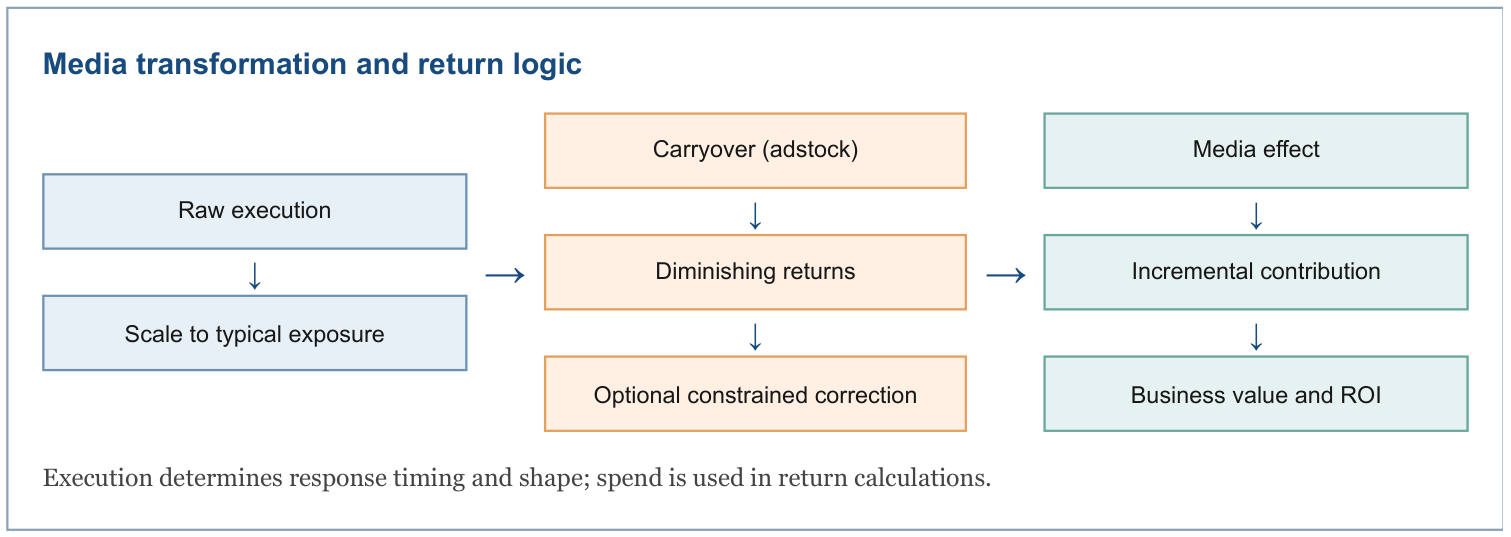
The model never applies a coefficient directly to raw spend. Raw execution is first scaled, carried through time, and saturated. A media coefficient therefore operates on transformed media pressure.

The pipeline for node $r$ is:

1. scale execution by its train-only typical positive level;
2. apply a causal finite-lag adstock kernel;
3. apply a bounded, zero-anchored saturation curve;
4. optionally blend the curve with a monotone, concave neural response;
5. multiply by an additive outcome-unit coefficient or a multiplicative log-effect coefficient.

Execution and spend have distinct roles. Execution identifies response shape and timing; spend is the denominator in ROI and, in the additive form, participates in the business-scale ROI parameterization.

---

Adstock, retention, and half-life

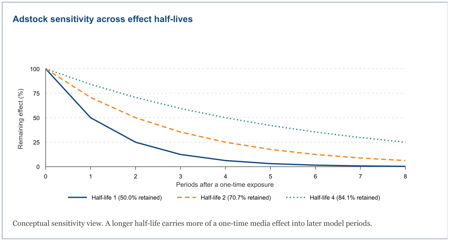
Adstock encodes the fact that media pressure can persist after execution.

Geometric adstock

For retention $0 \le \rho_r < 1$ and maximum lag $L$, normalized weights are

Formula

Each lag receives a decaying carryover weight, and all lag weights are divided by their total so they sum to one.

$$w_{r,l} = \frac{\rho_r^{\,l}}{\sum_{j=0}^{L} \rho_r^{\,j}}, \qquad l = 0,\dots,L.$$

Terms: $w_{r,l}$ is media node $r$'s weight at lag $l$; $\rho_r$ is retention; $L$ is the maximum lag; $j$ indexes all included lags.

The carried exposure is

Formula

Adstocked exposure is the weighted sum of current and previous scaled exposures.

$$a_{tgr} = \sum_{l=0}^{L} w_{r,l}\, \tilde{x}_{t-l,g,r},$$

Terms: $a_{tgr}$ is adstocked exposure; $w_{r,l}$ is the weight at lag $l$; $\tilde{x}_{t-l,g,r}$ is scaled exposure $l$ periods earlier.

with unavailable pre-history treated as zero. Normalization keeps a constant input on a comparable scale across retention settings.

The half-life $h_r$, in model periods, is related to retention by

Formula

Retention is chosen so that the remaining media effect falls to one half after the stated half-life.

$$\rho_r = 2^{-1/h_r},$$

Terms: $\rho_r$ is per-period retention for media node $r$; $h_r$ is its effect half-life measured in model periods.

with $\rho_r = 0$ when the configured half-life is zero. Retention can also be configured directly; a direct retention specification takes precedence.

Weibull adstock

Weibull adstock supports a delayed peak. For shape $k_r > 0$ and scale $\lambda_r > 0$, define survival at lag $l$ as

Formula

Remaining carryover at a lag is an exponential decay whose timing is controlled by Weibull scale and shape.

$$Q_r(l) = \exp\!\left[-\left(\frac{l}{\lambda_r}\right)^{k_r}\right].$$

Terms: $Q_r(l)$ is the remaining carryover at lag $l$; $k_r$ is Weibull shape; $\lambda_r$ is Weibull scale; $r$ identifies the media node.

Unnormalized lag mass is

Formula

The effect assigned to a lag equals the drop in remaining carryover from that lag to the next.

$$v_{r,l} = Q_r(l) - Q_r(l+1),$$

Terms: $v_{r,l}$ is unnormalized effect mass at lag $l$; $Q_r(l)$ and $Q_r(l+1)$ are remaining carryover at consecutive lags.

and the finite-lag weights normalize $v_{r,l}$ over $0,\dots,L$. The same causal convolution used for geometric adstock then produces $a_{tgr}$.

Configuration and estimation

The default maximum lag is 8 periods. Adstock parameters can be fixed or given priors, and can be estimated at media-node or parent-group scope. Default prior settings include a 2-period geometric half-life median, Weibull shape median 1.5, and Weibull scale median 3. These are prior centers, not hard-coded fitted values.

---

Saturation and diminishing returns

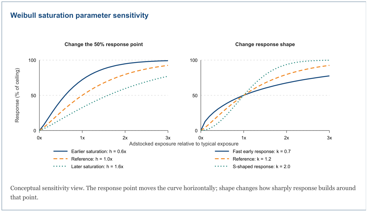
Saturation maps non-negative adstocked pressure $a$ to a bounded response. Every implemented family starts at zero. The discrete family is selected in the model specification and compared across candidates outside NUTS.

Weibull-CDF saturation

The default is

Formula

Saturated response equals one minus the remaining unrealized response; exposure is measured relative to the half-response point and curved by the shape parameter.

$$S(a;h,k) = 1 - \exp\!\left[-\log(2)\left(\frac{\max(a,0)}{h}\right)^{k}\right],$$

Terms: $S(a;h,k)$ is the response between zero and one; $a$ is adstocked exposure; $h$ is the 50% response point; $k$ controls curve shape; $\max(a,0)$ prevents negative exposure.

where $h > 0$ is exactly the 50% response point and $k > 0$ controls shape:

Formula

At exposure equal to the half-response point, the modeled response is exactly 50% of its ceiling.

$$S(h;h,k) = 0.5.$$

Terms: $S$ is the saturated response; $h$ is the 50% response exposure; $k$ is the curve-shape parameter; 0.5 means half of maximum response.

The default prior medians are $h = 0.75$ typical exposure and $k = 1.2$.

Anchored logistic saturation

Let midpoint $m > 0$, slope $s > 0$, and

Formula

The anchor value is the ordinary logistic response at zero exposure.

$$q = \frac{1}{1 + \exp(sm)}.$$

Terms: $q$ is the zero-exposure anchor; $m$ is the logistic midpoint; $s$ is the slope; $\exp$ is the exponential function.

The zero-anchored logistic response is

Formula

Start with the logistic response, subtract its zero-exposure value, and rescale it so response begins at zero and approaches one.

$$S(a;m,s) = \frac{\left[1 + \exp\!\big(-s(a-m)\big)\right]^{-1} - q}{1 - q}.$$

Terms: $S(a;m,s)$ is the zero-anchored response; $a$ is adstocked exposure; $m$ is the midpoint; $s$ is the slope; $q$ is the zero-exposure anchor.

Subtracting and rescaling by $q$ makes $S(0) = 0$.

---

Constrained neural response layer

The neural component is a small shape-constrained correction to the parametric saturation response. It is not an unrestricted residual network and does not bypass the Bayesian model.

Let $z \in [0,1]$ be the selected parametric saturation response for a parent media group. For neural unit $j$, define

Formula

Each neural basis converts the parametric response into a smooth increasing curve that starts at zero and is normalized to one.

$$B_j(z) = \frac{\mathrm{softplus}(b_j) - \mathrm{softplus}(b_j - s_j z)}{\mathrm{softplus}(b_j) - \mathrm{softplus}(b_j - s_j)},$$

Terms: $B_j(z)$ is the basis-unit response; $z$ is the parametric saturation response; $b_j$ is the unit bias; $s_j$ is a positive unit slope; softplus is a smooth positive transformation.

where $s_j = \mathrm{softplus}(\tilde{s}_j) + 10^{-4} > 0$. Each basis is zero-anchored, normalized at one, monotone, and concave. The neural curve is

Formula

The neural curve is a weighted average of all basis curves, with positive weights that sum to one.

$$n(z) = \sum_{j=1}^{J} w_j\, B_j(z), \qquad w_j = \mathrm{softmax}(\tilde{w})_j.$$

Terms: $n(z)$ is the combined neural curve; $J$ is the number of units; $B_j(z)$ is unit $j$'s basis response; $w_j$ is its normalized weight; $\tilde{w}$ is the raw weight vector.

The final transformed response is a shrinkage blend:

Formula

Final response blends the original parametric curve with the neural correction; the blend weight controls how much correction is allowed.

$$N(z) = (1-\lambda)\, z + \lambda\, n(z), \qquad 0 \le \lambda \le 1.$$

Terms: $N(z)$ is the final corrected response; $z$ is the original parametric response; $n(z)$ is the neural curve; $\lambda$ is the blend weight from zero to one.

The default has two units and $\lambda \sim \mathrm{Beta}(1,9)$, strongly favoring the parametric curve unless the likelihood supports a correction. Weight logits and raw slopes use Normal(0, 0.5) priors; biases use Normal(0, 1). One weight logit is fixed as a reference for identifiability.

All non-fixed neural parameters are sampled jointly by NUTS. Their posterior uncertainty therefore propagates into media response, contributions, ROI, and predictions. Setting use_neural_correction=False makes $N(z) = z$.

---

Additive versus multiplicative specification

Property	Additive	Multiplicative log-link
Outcome support	Real-valued outcome scale	Strictly positive fitting outcome
Media effect	Outcome-unit increment	Positive proportional lift
Likelihood	Student-t on standardized outcome	LogNormal or contaminated LogNormal
Primary media prior	Business-scale ROI	Positive transformed-media coefficient
Node contribution	$\beta_r r_{tgr}$	Full prediction minus channel-removal counterfactual
Decomposition additivity	Exact	Requires separate conserving allocation
Baseline dependence	Same absolute lift at same response	Lift grows with baseline level

Multiplicative counterfactual contribution

Let

Formula

Full prediction is the model's expected outcome with all variables included.

$$\hat{y}_{tg} = E[y_{tg} \mid \Theta]$$

Terms: $\hat{y}_{tg}$ is the full expected prediction; $y_{tg}$ is the outcome; $\Theta$ represents all fitted model parameters.

and let $\hat{y}^{(-r)}_{tg}$ be the expected prediction after removing $\ell_{tgr}$ while holding all other posterior values fixed. Then

Formula

A media node's removal contribution is full prediction minus the prediction with that node removed.

$$C^{CF}_{tgr} = \hat{y}_{tg} - \hat{y}^{(-r)}_{tg}.$$

Terms: $C^{CF}_{tgr}$ is the counterfactual contribution; $\hat{y}_{tg}$ is the full prediction; $\hat{y}^{(-r)}_{tg}$ is the prediction with media node $r$ removed.

Individual removal effects overlap under a log link, so they do not sum exactly to the total lift. For decomposition charts, the implementation also emits a conserving allocation:

Formula

Total media lift is divided among nodes in proportion to each node's log lift so allocated contributions add back to total lift.

$$C^{alloc}_{tgr} = \left(\hat{y}_{tg} - \hat{y}^{base}_{tg}\right) \frac{\ell_{tgr}}{\sum_{j} \ell_{tgj}},$$

Terms: $C^{alloc}_{tgr}$ is the conserving allocated contribution; $\hat{y}_{tg}$ is the full prediction; $\hat{y}^{base}_{tg}$ is the baseline-only prediction; $\ell_{tgr}$ is node $r$'s log lift; $j$ indexes all media nodes.

with a safe zero-effect convention. Counterfactual contribution is used for causal removal and ROI interpretation; conserving contribution is used where components must reconcile exactly to the predicted total.

Model form is an explicit candidate choice. Eligibility checks prevent use of the multiplicative form when its positive-outcome assumptions are not met.

---

Controls, external variables, and baseline

Controls are generic numeric variables supplied by the client. Price, promotion, distribution, holidays, macroeconomic factors, competitor activity, and supply variables are supported when they are mapped to controls at the model's time and geography grain. The model does not infer business semantics from the coefficient alone; semantic classification occurs during ingestion.

Baseline families

1. Linear: global intercept, centered geography offset, and linear trend.
2. Piecewise linear: linear trend plus equally spaced hinge bases. Hinge features are orthogonalized against intercept and trend and standardized on fitting periods.
3. Recent level: adds an indicator beginning at a configured fraction of the fitting window.
4. Dynamic AR(1): adds a recursively evolving latent state with bounded persistence and estimated innovation scale. The state is centered on fitting periods.
5. Local linear trend: recursively evolves level and slope innovations and orthogonalizes the result against intercept and linear trend.

Optional Fourier seasonality adds sine and cosine terms. The default seasonal period is 52 and the default number of harmonics is zero, so seasonality is enabled only when requested by the selected specification.

Holiday flags and similar controls are not special likelihood terms. They enter through standardized control columns. For additive models their effects are outcome-unit components after reversing target scaling. For multiplicative models they modify the log baseline and are reported through response-scale counterfactual removal.

---

Hierarchical and multi-level modeling

The implementation uses two distinct hierarchies.

Geography baseline hierarchy

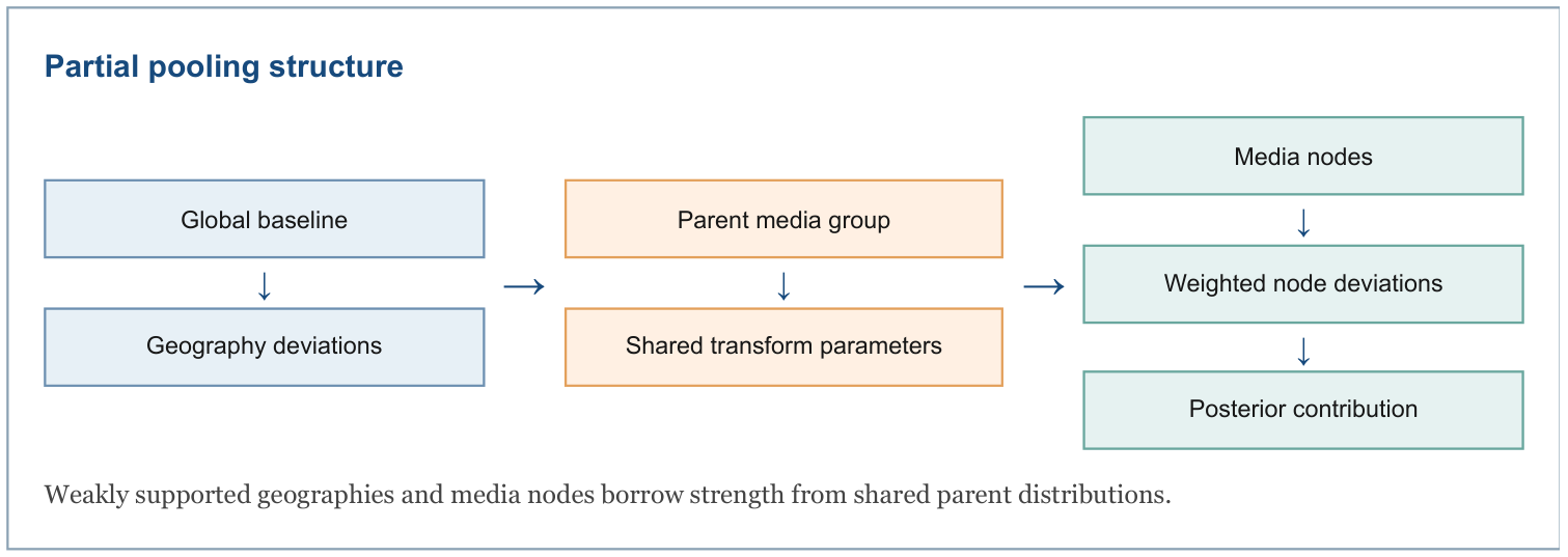
For $G > 1$, raw geography offsets use a non-centered parameterization:

Formula

Each geography starts with a standard-normal raw deviation, while a separate positive scale controls how different geographies may be.

$$\tilde{a}_g \sim \mathrm{Normal}(0,1), \qquad \sigma_a \sim \mathrm{HalfNormal}(0.5),$$

Terms: $\tilde{a}_g$ is geography $g$'s raw deviation; $\sigma_a$ is the common geography variation scale; 0 and 1 are the standard-normal mean and scale; 0.5 is the prior scale for geography variation.

Formula

Final geography effect equals the common variation scale times that geography's raw deviation after removing the average raw deviation.

$$a_g = \sigma_a\left(\tilde{a}_g - \frac{1}{G}\sum_{j} \tilde{a}_j\right).$$

Terms: $a_g$ is the centered geography effect; $\sigma_a$ is the geography variation scale; $\tilde{a}_g$ is the raw geography deviation; $G$ is the number of geographies; $j$ indexes all geographies.

One raw reference element is fixed before centering. This separates the global level from geography deviations and partially pools low-information regions. For a single geography, the deviation is zero.

Media-node hierarchy

The model is dimension-name agnostic. A media node may represent a channel, vehicle, campaign, creative, or another ingested entity. Every node maps to a parent pooling group. Transform parameters may be shared at parent-group scope or estimated at media-node scope. Media effects use group shifts plus weighted node deviations.

An identification analysis assigns each node one of these operational states:

• individually estimable;
• estimable with partial pooling;
• group only;
• unsupported.

The analysis uses active-period coverage, number of active periods, coefficient of variation, unique positive values, pairwise correlation, variance inflation factor, and spend support. Default warning thresholds include 5% active fraction, 6 active periods, 0.05 coefficient of variation, 0.95 pairwise correlation, VIF 10, and 3 unique positive values. Pooling begins earlier at correlation 0.80 or VIF 5 and can reduce the node deviation weight as low as 0.25 before moving to group-only attribution.

Product, retailer, or other business dimensions are supported when ingestion represents them in the canonical panel or media-node mapping. They are not separate hard-coded latent axes in the current model.