MMM: Methodology

Priors and Bayesian parameterization

Priors regularize weakly identified MMM components and provide a formal place for defensible business evidence. Defaults can be replaced with fixed values or reviewed custom priors through the model specification.

Positive and bounded parameters

Positive transform parameters use

Formula

A positive parameter is given a log-normal prior centered on the chosen median with stated log-scale uncertainty.

$$\theta \sim \mathrm{LogNormal}(\log m, \sigma_{log}),$$

Terms: $\theta$ is a positive model parameter; $m$ is its prior median; $\sigma_{log}$ is prior uncertainty on the log scale; $\sim$ means "modeled as distributed according to."

where $m$ is the prior median. Probabilities such as retention and neural blend weights use Beta priors. These parameterizations enforce valid domains without post-sampling clipping.

Baseline and control priors

Parameter	Default prior or scale
Global intercept $\alpha$	Normal(0, 1)
Geography scale	HalfNormal(0.5)
Geography raw offsets	Normal(0, 1), centered
Linear trend coefficient	Normal(0, 0.25)
Control coefficients	Normal(0, 0.25)
Piecewise trend-change raw coefficients	Normal(0, 1), multiplied by 0.10
Recent-level raw coefficient	Normal(0, 1), multiplied by 0.25
Dynamic AR persistence	0.95 x Beta(4, 2)
Dynamic AR innovation scale	HalfNormal(0.05)
Local-level innovation scale	HalfNormal(0.04)
Local-slope innovation scale	HalfNormal(0.01)
Seasonal coefficients	Normal(0, 1), multiplied by 0.10

Additive ROI hierarchy

The additive model uses a business-scale ROI prior for every media node. If $m^{ROI}_r$ and $s^{ROI}_r$ are the submitted log-prior location and scale, then

Formula

A node's log ROI equals its submitted prior center plus its parent-group shift plus a scaled node-specific deviation.

$$\log ROI_r = m^{ROI}_r + \delta_{p(r)} + s^{ROI}_r\, \epsilon_r.$$

Terms: $ROI_r$ is ROI for media node $r$; $m^{ROI}_r$ is the submitted log-prior center; $\delta_{p(r)}$ is the parent-group shift; $s^{ROI}_r$ is the submitted prior uncertainty; $\epsilon_r$ is the node deviation.

The parent-group shifts $\delta_p$ are centered and use a default scale of 0.15. The node deviations $\epsilon_r$ are non-centered, shrunk, and weighted by the adaptive pooling plan. A group-only node receives no unsupported unique deviation.

The coefficient is derived from ROI rather than sampled independently:

Formula

First total the business-valued transformed response. Then choose the effect coefficient so modeled profit contribution divided by spend equals the sampled ROI.

$$D_r = \sum_{t,g} M_{tg}\, r_{tgr}\, q_{tg}, \qquad \beta_r = \frac{ROI_r\, S_r}{\max(D_r, \varepsilon)},$$

Terms: $D_r$ is total business-valued response support; $M_{tg}$ is the fitting mask; $r_{tgr}$ is the transformed response; $q_{tg}$ is business value per outcome unit; $\beta_r$ is the effect coefficient; $ROI_r$ is node ROI; $S_r$ is fitting-period spend; $\varepsilon$ is a small positive safeguard against division by zero.

where $S_r = \sum_{t,g} M_{tg}\, s_{tgr}$ is fitting-period spend. This guarantees ROI reconciliation by construction.

Multiplicative media-effect priors

The multiplicative model samples positive log-effect coefficients. The default is a LogNormal prior with median 0.1 and log-scale 0.7. A HalfNormal family is also supported. Parameters can be defined per media node or parent group. A group-level coefficient can receive centered node-level multiplicative deviations with a HalfNormal(0.35) local scale.

The coefficient is not a raw spend-to-outcome multiplier. It multiplies the fully transformed response and represents log-scale lift.

Fixed values and business-informed priors

Transform and effect parameters may be fixed where externally validated evidence exists. Otherwise, user inputs define prior centers and uncertainty, not immutable curves. Evidence source and validity period belong to the input contract and reporting metadata, while NUTS updates non-fixed parameters using the observed likelihood.

---

Bayesian inference engine

Naukr AI MMM uses NumPyro on JAX and samples the continuous posterior with the No-U-Turn Sampler (NUTS), an adaptive Hamiltonian Monte Carlo algorithm.

NUTS uses gradients of the log posterior to propose distant states efficiently, reducing the random-walk behavior of simpler samplers. Warm-up adapts the step size and mass matrix; retained draws then represent the posterior distribution.

Runtime controls

The low-level run_inference API defaults to:

• 500 warm-up iterations;
• 500 retained draws per chain;
• 2 chains;
• target acceptance probability 0.90;
• maximum tree depth 10;
• random seed 2026.

The orchestration layer has independent configurable defaults of 300 warm-up iterations, 300 draws, and 2 chains so candidate and final runs can be sized separately. Production deployments should set these deliberately.

The implementation uses NumPyro's default initialization behavior. It does not define a custom initializer. JAX performs automatic differentiation and JIT compilation on the active CPU, GPU, or TPU backend. Chains run in parallel when the local device count permits and sequentially otherwise.

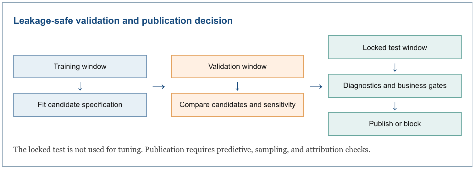
Discrete choices such as additive versus multiplicative, adstock family, saturation family, baseline family, lag length, and neural-correction use are not sampled inside NUTS. They are represented as candidate specifications and compared using leakage-safe validation.

---

Likelihood and observation model

Additive likelihood

For observed cells,

Formula

The standardized observed outcome is modeled around the standardized expected outcome using a robust Student-t error distribution.

$$\tilde{y}_{tg} \sim \mathrm{StudentT}(\nu, \tilde{\mu}_{tg}, \sigma),$$

Terms: $\tilde{y}_{tg}$ is the standardized observed outcome; $\tilde{\mu}_{tg}$ is the standardized expected outcome; $\nu$ is degrees of freedom controlling tail heaviness; $\sigma$ is the residual scale.

with

Formula

Residual scale receives a positive half-normal prior, while Student-t degrees of freedom are kept above two using an exponential prior.

$$\sigma \sim \mathrm{HalfNormal}(0.5), \qquad \nu = 2 + \nu_0, \qquad \nu_0 \sim \mathrm{Exponential}(0.1).$$

Terms: $\sigma$ is the residual scale; 0.5 is its prior scale; $\nu$ is Student-t degrees of freedom; $\nu_0$ is a positive offset; 0.1 is its exponential rate.

The Student-t likelihood is robust to occasional large residuals while keeping the conditional mean defined because $\nu > 2$.

Multiplicative likelihood

The ordinary multiplicative likelihood is

Formula

Positive observed outcome follows a log-normal distribution centered on expected log outcome, with positive log-scale noise.

$$y_{tg} \sim \mathrm{LogNormal}(\eta_{tg}, \sigma_{log}), \qquad \sigma_{log} \sim \mathrm{HalfNormal}(0.25).$$

Terms: $y_{tg}$ is the observed positive outcome; $\eta_{tg}$ is the expected log outcome; $\sigma_{log}$ is log-scale residual noise; 0.25 is its prior scale.

An optional contaminated LogNormal likelihood mixes a regular component and a wider component. The default outlier probability is 0.05 and the default scale multiplier is 4. Component locations are adjusted so both components preserve the same response-scale conditional mean. This separates occasional heavy-tail noise from systematic media lift.

Only cells selected by the observation mask enter the likelihood.

---

Model diagnostics and validation

Sampling diagnostics

• R-hat compares within-chain and between-chain variation. Values near one indicate that chains mixed to a common stationary distribution. The default gate requires maximum R-hat no greater than 1.01.
• Effective sample size (ESS) estimates the number of independent-equivalent posterior draws after autocorrelation. The default minimum is 200.
• Divergences identify problematic HMC trajectories and posterior geometry. The gate requires zero divergences.

Weak sampler diagnostics are resolved back to media node, parent group, geography, or control labels when possible.

Predictive metrics

Given posterior-mean prediction $\hat{y}_i$ over an evaluation mask:

Formula

RMSE is the square root of the average squared prediction error, so larger mistakes receive more weight.

$$RMSE = \sqrt{\frac{1}{n}\sum_{i} (\hat{y}_i - y_i)^2},$$

Terms: $RMSE$ is root mean squared error; $\hat{y}_i$ is the prediction; $y_i$ is the actual outcome; $n$ is the number of evaluated observations; $i$ indexes observations.

Formula

MAE is average absolute error. WMAPE is total absolute error divided by total absolute actual outcome.

$$MAE = \frac{1}{n}\sum_{i} |\hat{y}_i - y_i|, \qquad WMAPE = \frac{\sum_{i} |\hat{y}_i - y_i|}{\sum_{i} |y_i|},$$

Terms: $MAE$ is mean absolute error; $WMAPE$ is weighted mean absolute percentage error; $|\hat{y}_i - y_i|$ is absolute prediction error; $\sum_i |y_i|$ is total absolute actual outcome.

Formula

R-squared equals one minus model squared error divided by the squared error from always predicting the observed average.

$$R^2 = 1 - \frac{\sum_{i} (\hat{y}_i - y_i)^2}{\sum_{i} (y_i - \bar{y})^2}.$$

Terms: $R^2$ is the coefficient of determination; $\hat{y}_i$ is the prediction; $y_i$ is the actual outcome; $\bar{y}$ is the average actual outcome; $i$ indexes evaluated observations.

R-squared is not clipped, so it preserves its standard diagnostic meaning. The implementation reports overall point metrics, within-geography temporal fit after removing geography levels, and national aggregate time-series fit.

Posterior predictive interval diagnostics include empirical coverage and mean interval width. Validation-only interval calibration can add an absolute expansion learned from validation residuals; the locked test is never used to tune the interval.

Temporal validation

The pipeline supports:

• a chronological train, validation, and locked-test split;
• expanding-window rolling-origin folds;
• an optional balanced geography-time validation mask while preserving the final chronological test;
• simple leakage-safe forecast benchmarks;
• peak-capture diagnostics for material aggregate levels and changes;
• ROI reconciliation and prior-sensitivity checks.

Candidate specifications must pass configured acceptance gates before ranking. Accepted candidates are ranked primarily by validation WMAPE, followed by peak capture, temporal and national R-squared, overall R-squared, RMSE, interval width, and deterministic specification tie-breakers.

Attribution stability

The sensitivity run widens the active media prior and compares posterior mean profit-contribution shares. It reports maximum and mean absolute share changes. For additive models, ROI prior uncertainty is widened. For multiplicative models, the active log-effect prior is widened. This tests whether attribution depends excessively on one prior width.

---

Model identifiability and constraints

The implementation uses multiple complementary safeguards:

1. Media execution is scaled by train-only typical exposure to improve geometry.
2. Adstock, saturation, neural, and multiplicative-effect parameters are constrained to valid domains.
3. Additive media effects are positive because ROI is log-parameterized.
4. Multiplicative media coefficients are positive.
5. Geography and media hierarchies share information through partial pooling.
6. Centered hierarchy deviations prevent duplication of the global or group level.
7. Adaptive pooling suppresses unsupported node-level deviations rather than silently treating them as independently identified.
8. Collinearity and support diagnostics use pair correlations, VIF, activity, unique values, variation, and spend.
9. The neural correction is monotone, concave, zero-anchored, normalized, and shrunk toward the parametric curve.
10. Baseline changepoint and latent-trend bases are centered or orthogonalized against simpler trend terms.
11. Train-only preprocessing and locked testing prevent leakage.
12. Source-readiness checks require reviewed semantic roles, time-grain alignment, timestamp basis, and independent evidence where configured.
13. Publication artifacts carry attribution status, pooling weight, prior versus posterior movement, and quality flags.

These mechanisms reduce unreasonable solutions but do not create information that is absent from the data. Strongly correlated or low-support media may only be interpretable at their parent-group level.